Section 7 Analysing Spatial Autocorrelation with Moran’s I

Since the sample in 2019 & 2020 is too small to run a good result, you can analysis the autocorrelation based on the samples which contain these two years.

7.1 Generate the data for analysis

This process is similar to the 4.2 and 4.3 data preparation.

sdf = merge(London_Borough,df,by="GSS_CODE",all = TRUE)
sdf = sdf[,c("GSS_CODE","geometry","longitude","latitude")]
nsdf = sdf%>%
  add_count(GSS_CODE)%>%
  mutate(area=st_area(.))%>%
  mutate(density=n*1000*1000/area)

nsdf = dplyr::select(nsdf,density,GSS_CODE, n)

nsdf = nsdf%>%                    
  group_by(GSS_CODE)%>%         
  summarise(density = first(density), GSS_CODE = first(GSS_CODE))

## `summarise()` ungrouping output (override with `.groups` argument)

7.2 Centroids and neighbour list

Plot the centroids of all boroughs in London

coordsW = nsdf%>%
   st_centroid()%>%
   st_geometry()

## Warning in st_centroid.sf(.): st_centroid assumes attributes are constant over
## geometries of x

 plot(coordsW,axes=TRUE)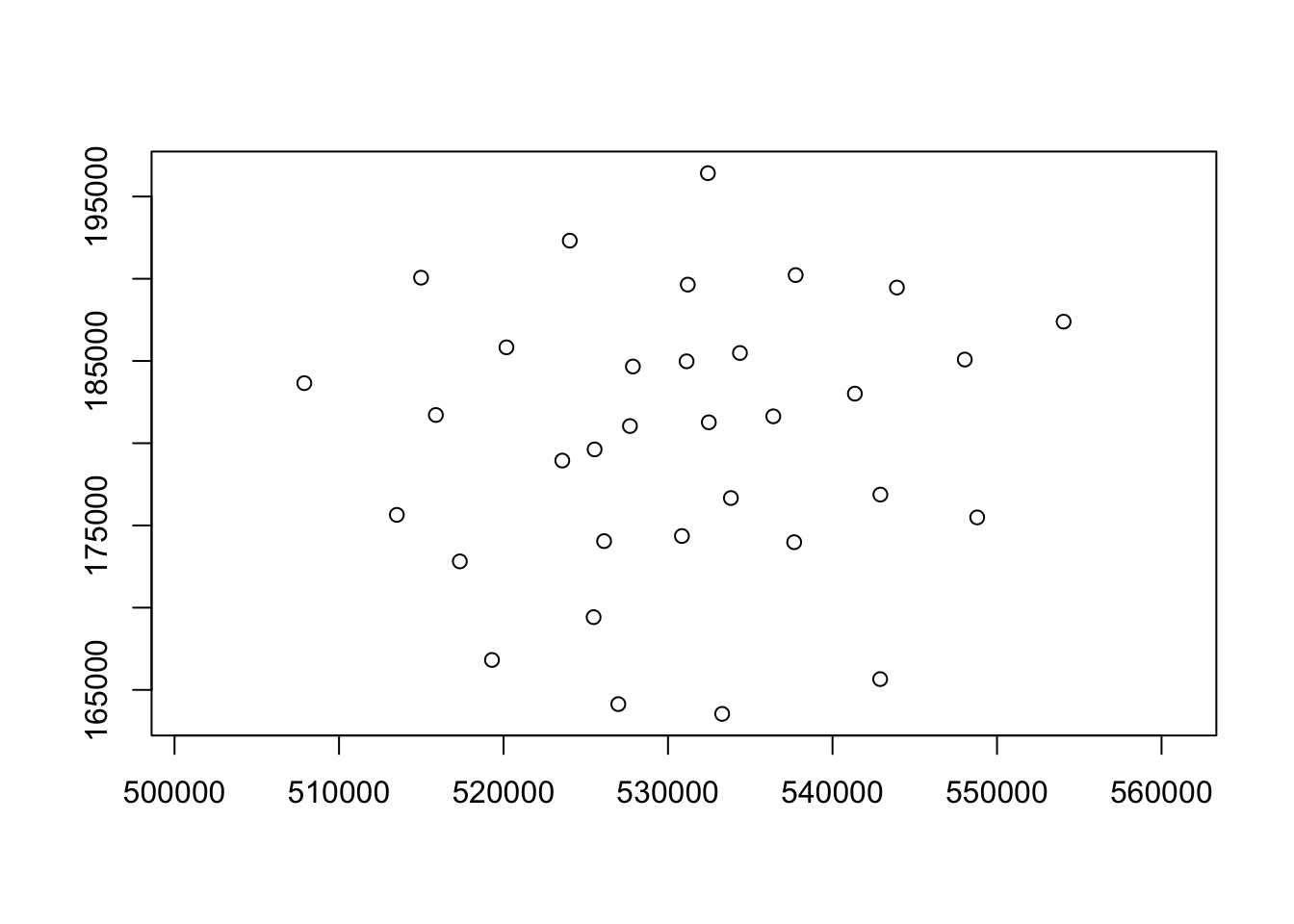

Create a neighbours list

 LWard_nb = nsdf %>% 
  poly2nb(.,queen=T)

Plot the neighbours list we create

plot(nsdf$geometry)
plot(LWard_nb, st_geometry(coordsW), col="blue", add = T)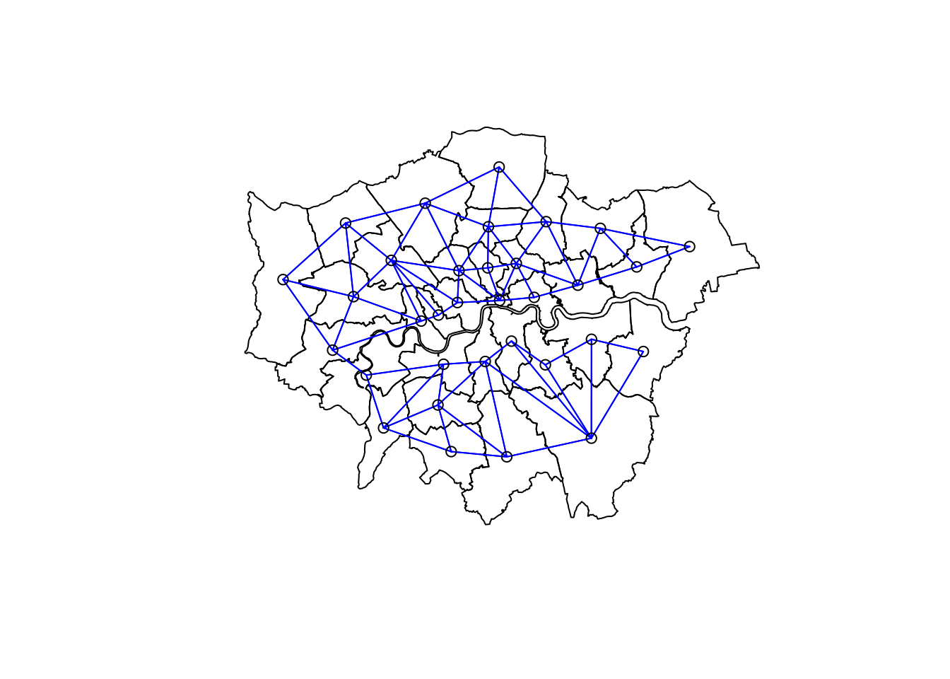

Create a spatial weights object from these weights, which can contribute to the further analysis autocorrelation analysis (Moran’s I test)

Lward.lw = nb2listw(LWard_nb, style="C")
head(Lward.lw$neighbours)

## [[1]]
## [1]  7 12 19 30 33
## 
## [[2]]
## [1] 16 25 26
## 
## [[3]]
## [1]  5  7 10 14 15
## 
## [[4]]
## [1]  6 11
## 
## [[5]]
## [1]  3  7  9 13 15 20 33
## 
## [[6]]
## [1]  4  8 11 22 23 28

7.3 Calculate the Global Moran’I Index

Conduct the global Moran’s I test to get the value.

 I_LWard_Global_Density = nsdf %>%
   pull(density) %>%
   as.vector()%>%
   moran.test(.,Lward.lw)
names(I_LWard_Global_Density)

## [1] "statistic"   "p.value"     "estimate"    "alternative" "method"     
## [6] "data.name"

head(I_LWard_Global_Density)

## $statistic
## Moran I statistic standard deviate 
##                         0.03513093 
## 
## $p.value
## [1] 0.4859877
## 
## $estimate
## Moran I statistic       Expectation          Variance 
##      -0.028283348      -0.031250000       0.007131055 
## 
## $alternative
## [1] "greater"
## 
## $method
## [1] "Moran I test under randomisation"
## 
## $data.name
## [1] ".  \nweights: Lward.lw    \n"

Conduct the Local Moran’s I test in these two years

 I_LWard_Local_Density = nsdf %>%
   pull(density) %>%
   as.vector()%>%
   localmoran(., Lward.lw)%>%
   as_tibble()

Merge the moran test result with the geometric dataset. The I value is stored in “density_Iz” and the Z value is stored in “density_Iz.”

nsdf<-nsdf%>%
   mutate(density_I = as.numeric(I_LWard_Local_Density$Ii))%>%
   mutate(density_Iz =as.numeric(I_LWard_Local_Density$Z.Ii)) 
summary(nsdf$density_I)
summary(nsdf$density_Iz)

7.4 Interactive visulisation of the distribution of the local Moran results

For drawing an interactive map, you should set “view” variables in tmap_mode function. You can set break box by the minimum and maximum value of Moran.

tmap_mode("view")

## tmap mode set to interactive viewing

#set the group and colour
summary(nsdf$density_Iz)

##      Min.   1st Qu.    Median      Mean   3rd Qu.      Max. 
## -1.813183 -0.007425  0.133178  0.046786  0.449411  0.975067

# breaks1 = seq(-3,1,0.5)
breaks1 = c(-2,-1,-0.1,-0.01,0,0.01,0.1,0.45,1,1.5 ) 
# breaks2 = c(-1000,-2.58,-1.96,-1.65,1.65,1.96,2.58,1000)
# Depends on the max and min value in Moran's I
MoranColours = rev(brewer.pal(8, "RdGy"))
# Plot the map
tm_shape(nsdf) +
  tm_polygons("density_Iz",
              style="fixed",
              breaks=breaks1,
              palette=MoranColours,
              midpoint=NA,
              title="Local Moran's I,EV charge points in London")

7.5 GI score

You can repeat the similar process as you can in 5.4 section to do the data preparation.

Gi_LWard_Local_Density = nsdf %>%
  pull(density) %>%
  as.vector()%>%
  localG(., Lward.lw)

# To get the Min and Max value
summary(Gi_LWard_Local_Density)

##    Min. 1st Qu.  Median    Mean 3rd Qu.    Max. 
## -0.8861 -0.4445 -0.1112  0.1998  0.4569  2.6561

Calculate the Gi score and transform the data type into numeric one.

Gi_nsdf = nsdf %>%
  mutate(density_G = as.numeric(Gi_LWard_Local_Density))

Based on the summary result of GI score to set the scale of breaks. Finally, the interactive map of Gi score distribution can be created.

GIColours = rev(brewer.pal(8, "RdBu"))

# This breaks box bases on the summary result：
#    Min. 1st Qu.  Median    Mean 3rd Qu.    Max. 
# -0.8861 -0.4445 -0.1112  0.1998  0.4569  2.6561 
breaks_GI = c(-2,-1.5,-1,-0.4,-0.2,0,0.2,0.5,1,2,2.5,3)

# Now plot on an interactive map
tmap_mode("view")

## tmap mode set to interactive viewing

tm_shape(Gi_nsdf) +
    tm_polygons("density_G",
        style="fixed",
        breaks=breaks_GI,
        palette=GIColours,
        midpoint=NA,
        title="Gi*, EV charge points in London")