Chapter 3 Methodology
3.1 Research Framework
The study area is 149 travel to work areas in England area (out of 228 in the UK). The areas in blue colour is the main research area (Figure 3.1). In this study, a data set containing all companies in UK will be cleaned and attribute selected, and technology companies will be identified and screened according to the classification and definition of technology companies on the official website of the British government. Before the quantitative study, this study is based on time and The spatial dimension counts the number of technology companies, and calculates the dynamic indicators of enterprise clusters and industrial combination indicators in a specific year and a specific region. Then this study conducts multiple regressions, univariate variables Moran index testing to conduct spatial quantitative research, and finally combines Qualitative spatial pattern trend research on the spatial changes of indicators in three different time periods(1998, 2008 and 2018).
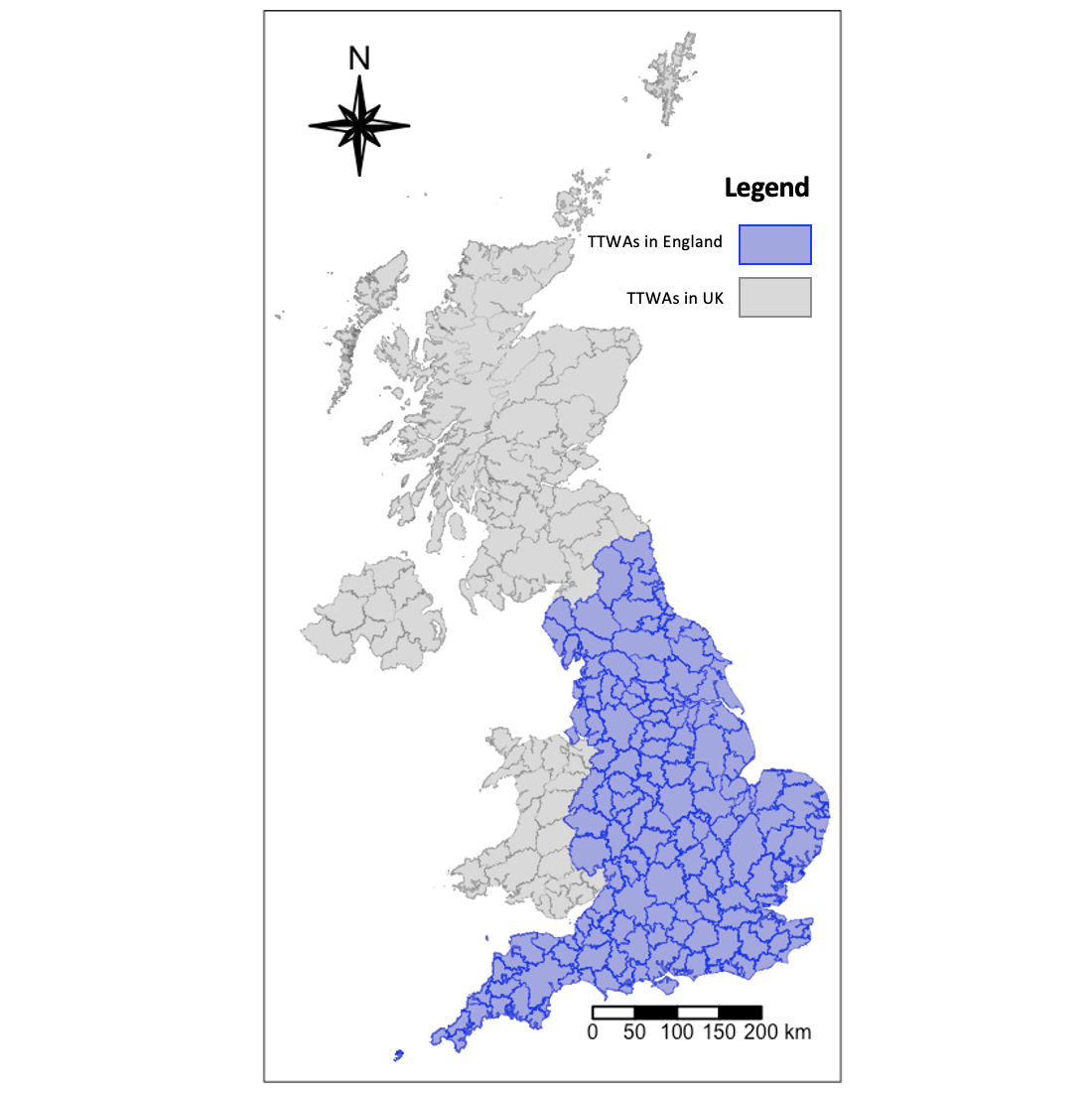
Figure 3.1: The Map of Travel to Work Areas (TTWAs) within UK
3.2 Data Source and Processing
This raw dataset is collected from the core company data from Open Corporates master company database (Open Corporates, 2018). And the size of dataset accounts for 15 GB which is handled with read_stata and get_chunk function to read large data file in chunks, then increasing the reading speed. The “primary uk sic 2007” identification field is the basis of industry finding and the “birth year” is the key to measure dynamics variables . All rows whose these two values are empty are removed(17% incorperate date is missing and sic code is complete). The details of data processing can be seen in the reproducible analysis reports in Appendix B.
3.3 Identifying Tech Clusters
For the identification of science and technology companies, this study introduces the main 2007 sic code table to judge the science and technology industry, referring to the classification method of the Science and Technology Classification data set on the ons.gov.uk website. In order to better identify science and technology companies for the UK. The economic contribution is officially based on the 2007 British Standard Economic Activity Classification, different data sources were combined to classify and label science and technology companies (Office for National Statistics, 2015).The 5-digital sic code can identify the economic activity classification of the technology industry in the finest granularity. The statistics bureau provided a comparison table of sic codes for the classification of science and technology industries, which can help this research to better identify technology companies from the big data of UK companies (3.1).
| 5-digit SIC07 code | Science and Technology category | Science and Technology topic |
|---|---|---|
| 26110 | Digital Technologies | Computer & Electronic manufacturing |
| 58210 | Digital Technologies | Digital & Computer Services |
| 62090 | Digital Technologies | Digital & Computer Services |
| 63110 | Digital Technologies | Digital & Computer Services |
| 27510 | Other scientific/technological manufacture | Electrical Machinery manufacturing |
| … | … | … |
| 86230 | Life Sciences & Healthcare | Healthcare services |
This research refers to the science and technology classification table provided by the government. The technology indicator is used to position the technology industry of all industries, and a total of 168 sic codes for the technology industry in 2007 were obtained, accounting for about 16% of all industry categories in the UK, including 5 industry categories such as Digital Technologies, Life Sciences and Healthcare, Publishing and Broadcasting , Other scientific/technological manufacture and Other scientific/technological services, details of the classification form will be attached in the attachment. There are almost 20% firms in the raw data belonging to tech firms according to the method of category as mentioned above.
3.4 Data Selection
3.4.1 Time Range (Temporal Dimension)
The reason why this research choose tech firms which incorporate from 1998 to 2018 is because the number of technology companies established in the UK in the past 20 years is significantly higher than before 1998, as shown in figure 3.2.
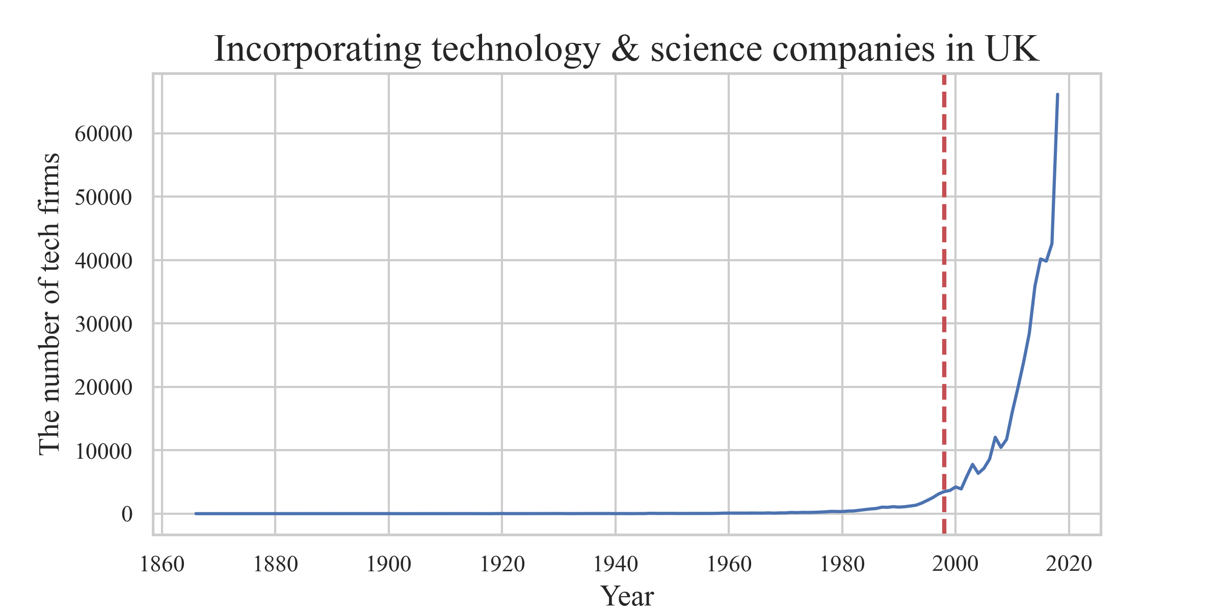
Figure 3.2: Incorporating technology and science companies in UK
3.4.2 Cluster Boundary (Spatial Dimension)
Travel to Work Locations is official statistics that capture local labour markets, i.e., areas where the majority (approximately 70%) of the people who live there work. These measures are based on responses to the 2011 and are used to define the TTWAs algorithmically. There are currently 228 TTWAs in the UK. When it is recognised that the activity of interest may be scattered across administrative boundaries such as local authority districts or NUTS areas, TTWAs are widely utilised in industrial clustering investigations (Prothero, 2021).
Relevant studies have shown that commuting across towns has become more common in England and Wales. People are not limited to living and working in the same administrative area. In addition, studies have found that low-skilled workers tend to rely on the public to work locally. Strong skill-oriented jobs are more dependent on cars, and they are also the main force for cross-city commuting. The technology industry has a greater demand for those strong skill-oriented workers which suggest that travel to work area(TTWA) is used as a cluster of technology companies compared to traditional administrative Region would be a good choice (Titheridge and Hall,2006). The University of Cambridge had funded some researchers to undertake the Wisbech 2020 Vision project to analyse the current problem, mining the potential future space for employment growth with alternative macro-economic scenario to help drive a high value-added growth plan in the local area (Burgess et al., 2014)
This geographical division can better reflect the relationship between population, company and work. In terms of geographic research, related researchers have combined the Business Structure Database (BSD) from the Office for National Statistics (ONS) and industry classification methods to use the ONS geographic area of TTWA to survey the commuting patterns and labour market of the population in 2011. Most scholars state that this might be an effective measure for the research of industrial clusters at the sub-regional level (Mateos-Garcia,2016).
3.5 Quatitative Analysis and Methods
3.5.1 Dynamics Measuring Index
Firm entry is the result of the interaction between the characteristics of an actor, on the one hand, and the surrounding environment, on the other hand (Frenken, Cefis and Stam, 2014).
To measure the degree of dynamic change of a cluster, it is necessary to calculate the entry rate of the technology cluster. Brandt used the enterprise’s entry rate and exit rate to measure the dynamics attributes of a company (2005). This research refers to the researcher’s calculation method. The number of enterprises entering and quitting a sector as a percentage of the total number of firms in the same sector in a given year is used to compute entry rate in this tech cluster dynamics research(ibid). The calculation method is as follows.
\[ Entry\ Rate_{i,t} = \frac{Incorporating\ Firms_{i,t}}{Total\ Firms_{i}} \]
where \(i\) means location(travel to work area), \(t\) means year
3.5.2 Industry Mix Measuring Index
It is necessary to calculate the Herfindahl-Hirschman Index or location quotient of the technology cluster to measure the degree of industrial concentration in a cluster area. However, only the former method is used because the employment data corresponding to the corresponding region year is missing; Here is a reference to the quantitative method of industrial concentration of Chao Lu’s research team (2017). HHI is calculated by squaring the market share of each competing company and then adding the results, where the market share is given in the form of scores or points (ibid). Increases in the Herfindahl index generally indicate a decrease in competition and an increase of market power, whereas decreases indicate the opposite (Hall et al., 2009), as the calculation method shown below.
\[ HHI_{\ i,t} = \sum_{j=1}^N (\frac{Tech\ Firms_{j,i,t}}{Total\ Tech\ Firms_{i,t}})^2 \] where
\(HHI_{i,t}\) means Herfindahl-Hirschman Index in location \(i\) and year \(t\)
\(N\) is the overall number of individual tech firm contained.
\(k\) represents the \(k\)th industry in location \(i\) and year \(t\).
\(Tech\ Firms_j\) is the number of j-th individual tech firm
\(Total\ Tech\ Firms\) represents the number of total tech firms in a specific location and year.
3.5.3 Regression
In order to quantify the impact of industry concentration and company density in the cluster on the cluster dynamic variable (entry rate), the Herfindahl-Hirschman Index and company density corresponding to the year and location(i.e. ttwa) in the data are used as independent variables (Table 3.2). And the variable of the numeric data type of entry rate is regarded as the dependent variable
| Independent Variables | Type | Description |
|---|---|---|
| Density | numeric | The density of tech firms |
| Herfindahl-Hirschman Index | numeric | The index measuring the industry mix |
| Year | category | Years from 1998 to 2018 |
| Location | category | Top ten clusters of companies in England |
Dynamics variable(entry rate) is measured empirically by the ratio of the number of new firms at the end of a period to the total number of firms at the beginning of the period(Hause and Du Rietz, 1984), unless otherwise stated. The equation regression model is given:
\[ \ y\ =\ b_0 + b_1 \ x_1 + b_2 \ x_2 + \sum_{i=3}^{4} \ b_i \ x_i + \epsilon_{i,j} \] where
\(y\) means entry rate in the year and location \(x_1\) means the year, a dummy variable \(x_2\) means location, i.e. travel to work area(TTWA) \(x_3\) means the density of tech firms in a specific year and location \(x_4\) means Herfindahl-Hirschman Index in in a specific year and location \(\epsilon_{i,j}\) is a random error.
3.5.4 Global Autocorrelation (Moran’s I)
One of the most popular and often used measures of spatial autocorrelation is Moran’s Index. Based on the locations and values of the feature, the Global Moran’s I tool analyzes the pattern of a data set spatially and decides if it is scattered, clustered, or random. The program calculates the Moran’s I Index value, as well as the z-score and p-value, to statistically validate the Index. It is computed using the formula below (Kumari and et al., 2019).
\[ Moran's \ I = \frac{n}{S_0} \frac{\sum_{x=1}^n \sum_{y=1}^n w_{x,y} z_x z_y}{\sum_{x=1}^n z_x^2} \] \[ S_0 = \sum_{x=1}^n \sum_{y=1}^n w_{x,y} \]
where \(z_x\) stands for deviation of an attribute from its mean \((x_i – X̅)\) for feature \(X\), \(w_{x,y}\) is the spatial weight among feature \(X\) and \(Y\), \(n\) is the total number of features and So is the summation of all spatial weights
The statistic’s \(z_j\) score is given below
\[ z_x = \frac{I - E[I]}{\sqrt{V[I]}} \] where
\[ E[I] = \frac{-1}{(n-1)} \]
\[ V[I] = E[I^2]-E[I]^2 \]
The Moran’s Index(I) has a range of values from -1 to 1. Index value 1 indicates that the observed pattern is spatially clustered. On the other hand value -1 indicates scattering or dispersion. Moran’s I assign a value of near or equal to zero to the lack of auto correlation. The z-score and p-value of the Index are only used to form final judgments regarding the observed pattern. Besides, local indicators of spatial association will be applied to measure the high-high and low-low clusters(Anselin, 2010). According to research method of Kumari’s team(2019), the Moran’s I of three time period will be calculated to analysis the dynamics change in spatial and temporal aspects.
3.5.5 Hot-Spot Analysis (Getis-Ord Gi*)
Only positive spatial autocorrelation is taken into account by the local Getis statistics, which allows for discrimination between clusters of similar values that are high or low relative to the mean. The Getis–Ord local statistics are calculated as follows by Getis and Ord (2010):
\[ G^*_j = \frac{\sum_{j=1}^nw_{i,j}x_j - \bar{X}\sum_{j=1}^{n}w_{i,j}}{S\sqrt{\frac{[n\sum_{j=1}^{n}w^2_{i,j} - (\sum_{j=1}^{n}w_{i,j})^2)]}{n-1}}} \]
where \(x_j\) is the attribute value for feature \(j, w_{i,j}\) is the spatial weight between feature \(i\) and \(j\), \(n\) is equal to the total number of features and:
\[ \bar{x} = \frac{\sum_{j=1}^{n}x_j}{n} \]
\[ S = \sqrt{\frac{\sum_{j=1}^{n}x^2_j}{n} -(\bar{x})^2} \]
The Gi* statistic returned for each feature in the dataset is a z-score (Getis and Ord, 2010). For statistically significant positive z-scores, the larger the z-score is, the more intense the clustering of high values (hot spot). For statistically significant negative z-scores, the smaller the z-score is, the more intense the clustering of low values (cold spot).
3.6 Limitations
In term of missing value in the original dataset, there are almost 99.8% missing value in dissolution date. This means that most companies do not have a dissolution date, which might not mean that some companies survive, nor can it accurately reflect the company’s exit numbers in a specific year and region. Moreover, the company’s incorporation date data (including firms birth year) is also missing about 17.26%. These two difficulties make the data after cleaning process may have the risk of insufficient accuracy in representing the dynamics of the industry. The model prediction after fitted to this dataset might not reach the same situation as the real world level.
England travel to work areas might not be a data-driven method to identify the clusters. This spatial boundary data is not an up-to-date dataset because it is lastly updated in 2015. Changes in commuting have pushed TTWA boundaries further since their inception in the 1980s. With the passage of time, the boundaries of TTWA will be further changed in the future due to changes in commuting methods(Ozkul,2014) which might make this research slightly inappropriate in the future application.
The value of this statistical data(Herfindahl-Hirschman Index) for identifying monopoly development, on the other hand, is directly dependent on the precise definition of a market (Kwoka, 1977). For instances, geographical considerations might influence market share. This dilemma can arise when there are nearly equal market share of tech businesses in a given sector, but they each operate exclusively in distinct regions of the travel to work area, resulting in each firm having a monopoly inside the specific marketplace in which it conducts business, which might make it more difficult to measure the industry mix in a specific location and year. Furthermore, one IT firm may control as much as 70% of the market for a certain area of the digital industry (i.e. the sale of one specific equipment). As a result, that company would have a near-total monopoly on the manufacturing and sale of that commodity.
3.7 Ethical Statement
The data for this project comes from OpenCorporates, a firm that aggregates company-level data from around the world(https://opencorporates.com/). In this case, OpenCorporates have taken data from the UK Companies House register (https://www.gov.uk/government/organisations/companies-house). As detailed by Nathan and Rosso (2015), all limited companies in the UK need to registers with Companies House when they are set up, and provide annual returns and financial statements. These include details of directors and company secretary, registered office address, shares and shareholders, as well as company type and principal business activity. Thus, all the data used here is already in the public domain.
The research objectives are tech firms in the UK for this project and the individual data will not be collected and measured in this project. For issues of deanonymisation or privacy, traceable information such as the real companies name and ID will not be utilised in the research. The raw data will be cleaned and filtered by several key variables include industries instead of the company’s name or other sensitive information before doing the research. Through data cleaning, pre-processing, desensitisation or other processing methods, the risks of damage to company interests (such as social reputation, economic benefits and etc.) will be mitigated to an as low as possible level in the research process. Besides, this project will not cause discrimination of industries or job categories. The final analysis results, such as the different industry concentration in each region, will not deepen some people’s stereotypes and prejudices about the region (This content will be fully discussed in the project discussion section).
It is necessary to point out and declare the objectivity of the analysis and the non-absoluteness of the results in the disclaimer. Consider the feelings of people and governments in different parts of the UK, this research will prevent the influence of personal preferences and subjective emotions. Last but not least, the leakage of companies’ name and information will be protected. For example, in the reflection of the results section of academic research, the name and related information of the companies that moved may be revealed. Although this information may be open to the public you need to know that this information may be used by people with other ulterior motives. This project will desensitise the company name and information at the stage of chart presentation, such as using A, B, and C to replace them to achieve this purpose.