Chapter 4 Results
4.1 Spatial and Temporal Distribution
In terms of three variables’ change of overall England level,it can be found that the average firms’ entry rate and density in England increase significantly(Figure 4.1). There was a growth in firms entry rate from 0.01(1998) to 0.14(2018) and the statistics of density climb from 0.02 to 0.43 during these decades (Table 4.1). However, the Herfindahl-Hirschman index decreased by less than 0.1 in 2018 which is 1/3 times than that in 1998. Overall, it can be seen that the dynamics increased but the industry concentration reduced.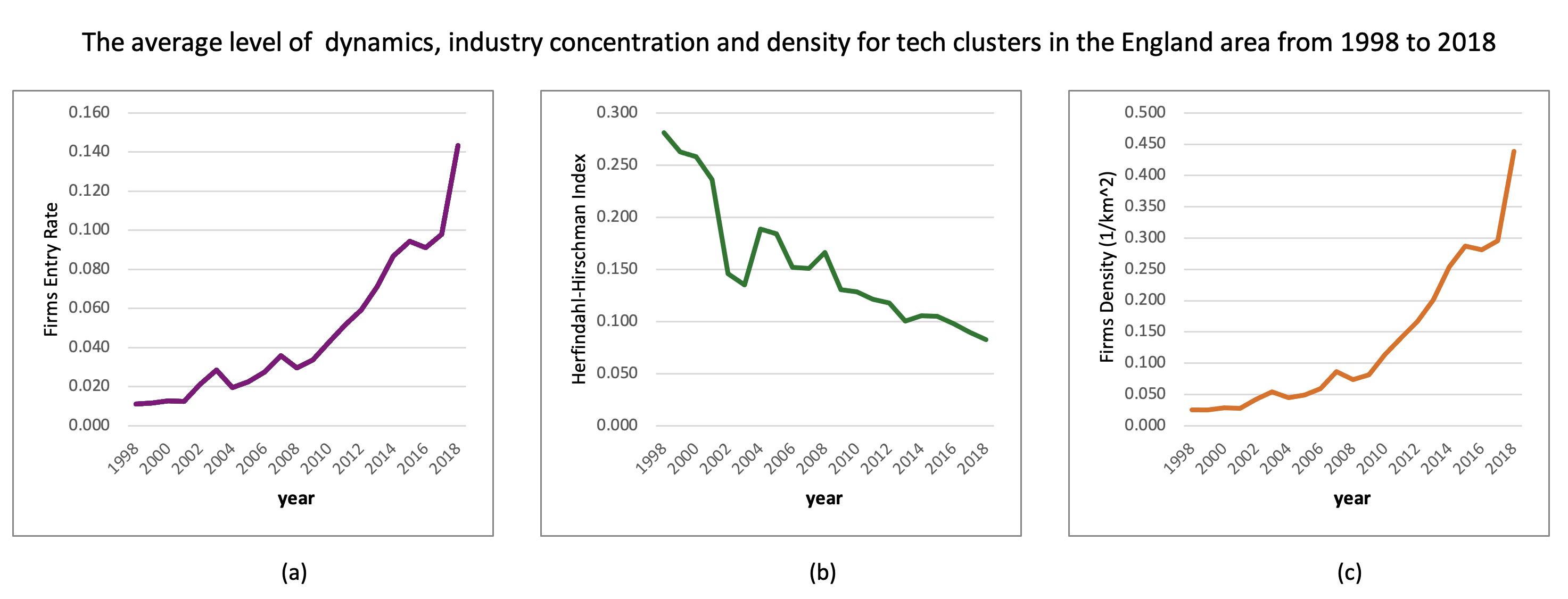
Figure 4.1: The average level change of three variables in two decades
| Year | Entry Rate | Herfindahl-Hirschman Index | Density (1/km^2) |
|---|---|---|---|
| 1998 | 0.0111338 | 0.2811410 | 0.0251467 |
| 1999 | 0.0116754 | 0.2625985 | 0.0255016 |
| 2000 | 0.0127544 | 0.2580325 | 0.0288208 |
| 2001 | 0.0124221 | 0.2361455 | 0.0279131 |
| 2002 | 0.0212760 | 0.1460459 | 0.0420549 |
| 2003 | 0.0285419 | 0.1350075 | 0.0540107 |
| 2004 | 0.0195123 | 0.1886668 | 0.0449568 |
| 2005 | 0.0225973 | 0.1841296 | 0.0492084 |
| 2006 | 0.0274033 | 0.1521901 | 0.0592952 |
| 2007 | 0.0358175 | 0.1507693 | 0.0862518 |
| 2008 | 0.0295100 | 0.1662619 | 0.0737782 |
| 2009 | 0.0336153 | 0.1305273 | 0.0817783 |
| 2010 | 0.0425260 | 0.1285513 | 0.1134154 |
| 2011 | 0.0516425 | 0.1212957 | 0.1404650 |
| 2012 | 0.0593572 | 0.1179875 | 0.1664194 |
| 2013 | 0.0712224 | 0.1006216 | 0.2015662 |
| 2014 | 0.0867586 | 0.1056914 | 0.2538923 |
| 2015 | 0.0943852 | 0.1048371 | 0.2869250 |
| 2016 | 0.0912387 | 0.0980931 | 0.2812983 |
| 2017 | 0.0979282 | 0.0894585 | 0.2954844 |
| 2018 | 0.1432780 | 0.0827082 | 0.4387067 |
4.1.1 Tech Cluster Dynamics
From 1998 to 2018, the entry rate of each travel to work area (TTWA) in England will change drastically every decades. For example, in 1998 the darker colored areas were mostly around the Greater London area and the entire southern part of England(Figure 4.2). The overall entry rate in 2008 was higher than that in 1998 and showed a trend of new companies entering the north of England. In this year, some travel to work areas on the edge of England have more prominent entry rates, such as Malton, Minehead and Bridport. However, the overall entry rate in 2018 was about twice as high as the average in 2008. Moreover, ttwa with high entry rate is mostly concentrated in the north and the surrounding areas of Greater London. The overall trend can be witnessed as given by table 4.1 that there is an increasing trend in the overall level of entry rate from 1998 (average about 1.06% ) to 2018 (average about 14.33%)
Finally, from the perspective of changes in temporal and spatial distribution, the increase in the entry rate of the travel to work area in the northern part of England is much larger than that in the southern part. The areas with high entry rates before 2008 were mostly scattered in other areas except for the Greater London area. However, close to after 2018, London and its surrounding areas, the central Manchester-Birmingham area and the southwest, such as Exeter, have a rising entry rate. In contrast, in 2008, the urban agglomerations north of Leeds had higher firm entry rates in tech industry(Figure 4.2).
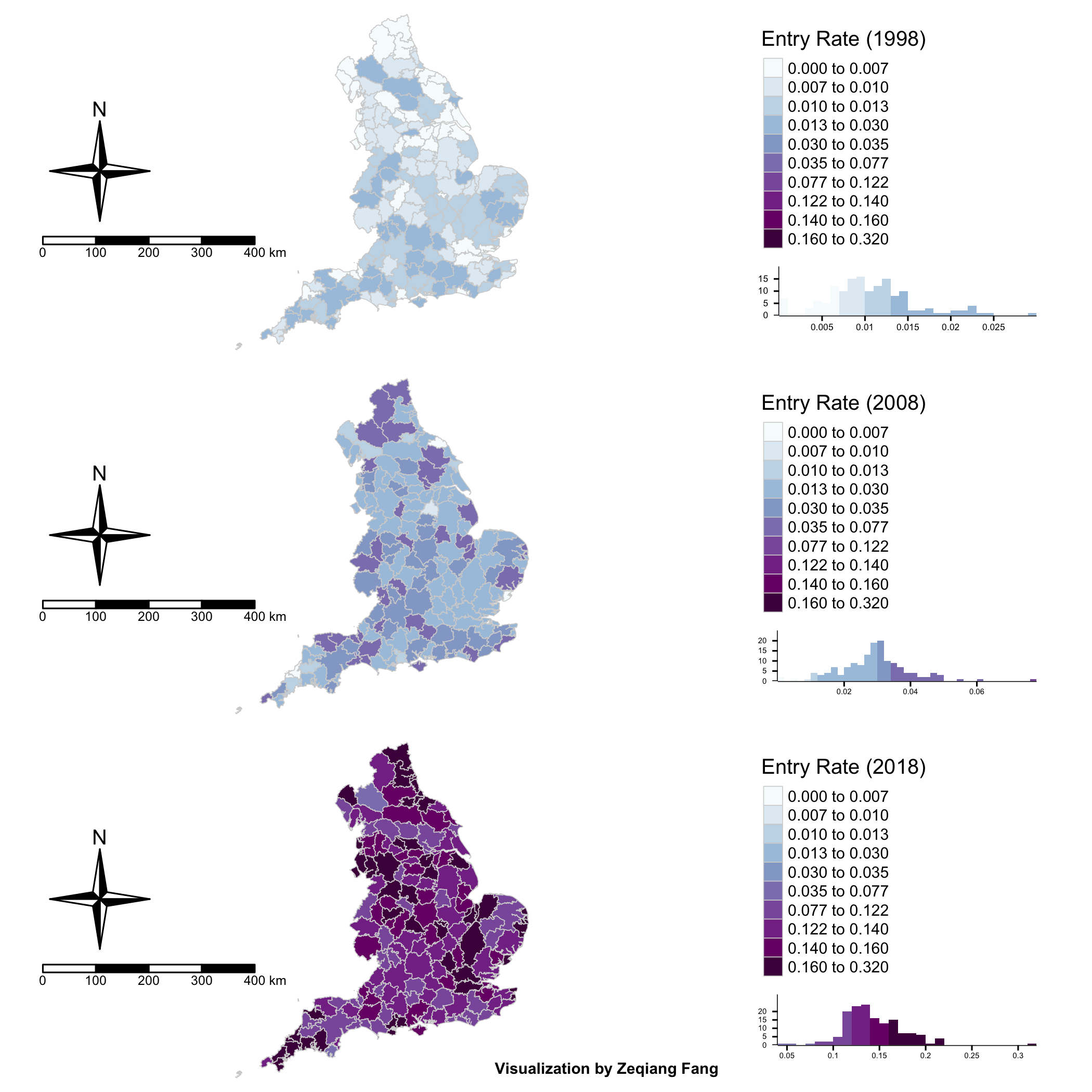
Figure 4.2: The Distribution of the Firms Entry Rate of the England Travel to Work Areas(TTWAs) from 1998 to 2018
4.1.2 Tech Industry Concentration
In terms of herfindahl-Hirschman index of tech industry in travel to work area of England. As given figure below, it can be seen that the Herfindahl-Hirschman index has a downward trend year by year (Figure 4.3). In the methodology module, this index is mentioned as a measure of industrial concentration. A decrease in the value represents an increase in industrial competition and a decrease in market power. The decline of the index means that the types of SIC codes corresponding to companies in a particular region have increased in a year or the number of companies corresponding to a large share of SIC codes has decreased. In other words, the types of technology industries corresponding to the unit area have increased, or the number of advantageous industries has decreased; you can see The concentration of technology industries out of England declined year by year from 1998 to 2018 (Table 4.1). In the same way, the diversity of the technology industry is also increasing, and the richness of the industry may also be related to the increase in the entry rate of enterprises.
From the perspective of temporal and spatial distribution, the technology industry was concentrated in northern England, northern and southwestern England before 2008. With the passage of time, even if the concentration of industries in some small areas scattered on the border of England is still high, the Herfindahl-Hirschman index in these places has gradually decreased to a level comparable to that of the Greater London area(Figure 4.3).
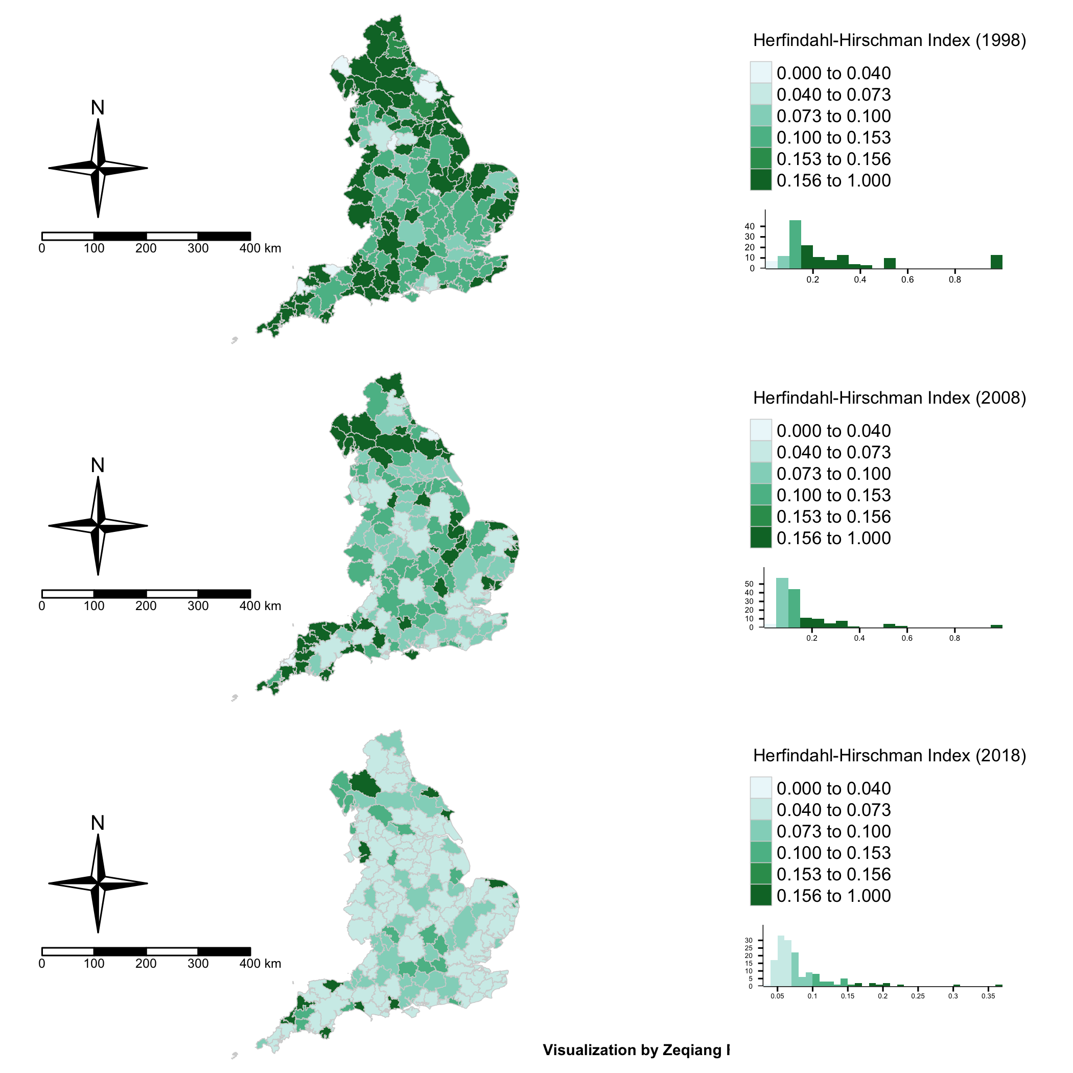
Figure 4.3: The Distribution of the Herfindahl-Hirschman Index of the England Travel to Work Areas(TTWAs) from 1998 to 2018
4.2 Regression Analysis
For 149 tech clusters(travel to work areas), the regression results can indicate the relationship among cluster dynamics, industry mix and firms density in different years(1998-2018) and locations (149 tech clusters). Among these three models, the model with outliers excluded and logarithmic processing of the dependent variable performed better. It can be seen that the Herfindahl-Hirschman index has a negative correlation with the tech cluster dynamic variable (entry rate) but the density has a positive effect.
Taking Model [3] as an example, every time this indicator decreases by one unit, the entry rate might increase by about \(e^{1.37}\) unit times higher than the original one. The high confidence of this coefficient can explain 99% of all observation data. On the contrary, for the density of these tech clusters in Model [3], every time the density increases by one unit, the corresponding dependent variable entry rate will be about \(e^{0.5}\) unit times more than the original one (Table 4.2). Although the HHI and Density values of the three models are not the same, the positive and negative effect of the relationship are similar. For example, for the industrial concentration variable HHI, all three models show a negative correlation (Table 4.2). And when HHI and Density change the same unit, the former seems to have a greater impact on the entry rate (it may increase the dependent variable entry rate by more than \(e\) times in both model 1 and model 2)
| Model | [1] | [2] | [3] |
|---|---|---|---|
| Method | OLS | OLS | OLS |
| Sample | all areas | all areas | exclude 2018 London |
| Dep. Variable | Entry Rate | Log(Entry Rate) | Log(Entry Rate) |
| HHI | -0.0281*** | -1.332*** | -1.3693*** |
| [0.002] | [0.045] | [0.044] | |
| Density | 0.0168*** | 0.3904*** | 0.504*** |
| [0.001] | [0.019] | [0.022] | |
| Constant | 0.0207* | -4.1138* | -4.0948* |
| [0.003] | [0.068] | [0.066] | |
| Observations | 3089 | 3089 | 3088 |
| R-squared | 0.89 | 0.89 | 0.90 |
| a All regressions include dummy variables for 149 travel to work areas(ttwa) in England and 20 years from 1998 to 2018. Figures in brackets are standard errors. , , and represent statistical significance at 1%, 5%, and 10%, respectively. | |||
| b HHI defined by Herfindahl-Hirschman index can indicate the industry concentration | |||
| c Source: tech firm data in England travel to work areas from 1998 to 2008 (n = 3089) |
As mentioned in the methodology section(Brandt, 2005), Table 4.3 can illustrates the unconditional relation between entry rate and tech cluster characters. These two independent variables are controlled to be added in the regression model which can help to observe to what extent they can have an influence on the dynamics element(entry rate).
When the year and regional conditions in the model remain unchanged, the model [1] only adds Herfindahl-Hirschman index to consider the regression analysis, and it can be found that the coefficient is about -1.2 and the confidence level is greater than 95%. Similarly, the model [2] only considers adding firm density into the fitting, the coefficient of this independent variable is about 0.38 and the statistical significance is also less than 5%. However, when other conditions are the same, adding two variables into the model[3] at the same time, the absolute value of each coefficient increases, and the confidence level increases, and the overall goodness of fit is also improved which can be seen in table @ref(tab :tab-regression-control-var).
In terms of Herfindahl-Hirschman index, the entry rate might decrease when this indicator increase. Consistent with model[2], the entry rate increase with density (Table 4.3). The HHI decrease and density increase, leading to lower entry rates.
| Model | [1] | [2] | [3] |
|---|---|---|---|
| Method | OLS | OLS | OLS |
| Sample | exclude 2018 London | exclude 2018 London | exclude 2018 London |
| Dep. Variable | Log(Entry Rate) | Log(Entry Rate) | Log(Entry Rate) |
| HHI | -1.1844** | -1.3693*** | |
| [0.047] | [0.043] | ||
| Density | 0.3779** | 0.504*** | |
| [0.025] | [0.022] | ||
| Constant | -4.1884* | -4.5143* | -4.0948* |
| [0.072] | [0.075] | [0.066] | |
| Observations | 3088 | 3088 | 3088 |
| R-squared | 0.884 | 0.869 | 0.901 |
| a All regressions include dummy variables for 149 travel to work areas(ttwa) in England and 20 years from 1998 to 2018. Figures in brackets are standard errors. , , and represent statistical significance at 1%, 5%, and 10%, respectively. | |||
| b HHI defined by Herfindahl-Hirschman index can indicate the industry concentration | |||
| c Source: tech firm data in England travel to work areas from 1998 to 2008 (n = 3089) |
4.3 Spatial Autocorrelation
Through the global Moran’s Index test of entry rate variable, it can be found that as time increases, the spatial cluster effect of entry rate attribute in England is getting weaker and weaker, from about 0.12 (1998) to 0.05 (2018).
The confidence of global Moran’s I in 1998 is as high as 95%. But the statistical significance of 2008 is lower than 10%, which indicates weak interpretability of these two years(Table 4.4).
| Year | Moran’s Index | p value | z-score |
|---|---|---|---|
| 1998 | 0.118 | 0.00 | 2.438 |
| 2008 | 0.062 | 0.08 | 1.348 |
| 2018 | 0.056 | 0.10 | 1.238 |
Contrary to the entry rate variable, the density attribute value of England has always maintained a relatively obvious spatial aggregation phenomenon, although the global Moran’s Index of the density variable has been decreasing year by year. This variable has higher confidence in global Moran’s I statistics in the three-year statistics, thus its interpretability is higher than that for mentioned entry rate (Table 4.5).
| Year | Moran’s Index | p value | z-score |
|---|---|---|---|
| 1998 | 0.436 | 0.00 | 10.078 |
| 2008 | 0.325 | 0.00 | 7.545 |
| 2018 | 0.189 | 0.00 | 4.982 |
4.3.1 LISA Analysis of Firms Dynamics
Local indicators of spatial association(LISA) according to the table 4.6, the z-score with its significance can be found.
| Z-score | p-value | confidence |
|---|---|---|
| less than -1.65 or more than 1.65 | less than 0.10 | 0.90 |
| less than -1.96 or more than 1.96 | less than 0.05 | 0.95 |
| less than -2.58 or more than 2.58 | less than 0.01 | 0.99 |
The visualisation result of the local Moran’s index’s z-score of Entry rate is as similarly indicated by the global Moran coefficient (Figure 4.2). With the growth of the year, the overall agglomeration effect of England has decreased. But, in this process, the agglomeration effect in the northern region was higher than that in other regions. However, the travel to work areas in the southwest corner changed significantly from the early cluster effect in 1998 to the corresponding outliers such as low-high, high-low areas in 2018 (Figure 4.4 ). In addition, from Figure 4.3, the higher industrial concentration in the north also makes the phenomenon of dynamics agglomeration more obvious than that in other places in England area.
To be more specific, high-high clusters in 1998 are mainly concentrated in travel to work areas in northern areas such as Newcastle, southern areas such as Andover-Newbury, and the southwest of Exeter. The entry rate values around these places may be higher than the British average. The low-low clusters of entry rates are clustered in the northern North Yorkshire area. The surrounding areas of these places usually have relatively close entry rates and low entry rate values.
The high-high cluster has shifted over time (the north like Whitehaven and the southwest corner like Launceston areas with higher entry rates gradually formed). By 2018, high-high cluster only appeared in travel to work areas around Liverpool, and new low tech firms entry rate areas were formed in Workington and Penrith&Appleby (Figure 4.4)
Central regions of England such as London, Birmingham and other regions have not had obvious spatial clustering effects in the visualisation results. This may be due to the low statistical confidence of the local Moran’s index among regions. Or it might be because the data in this study is aggregated before calculated. The related data may be missing after the HHI and entry rate are utilised, which might not perfectly represent the company information in some parts of England.
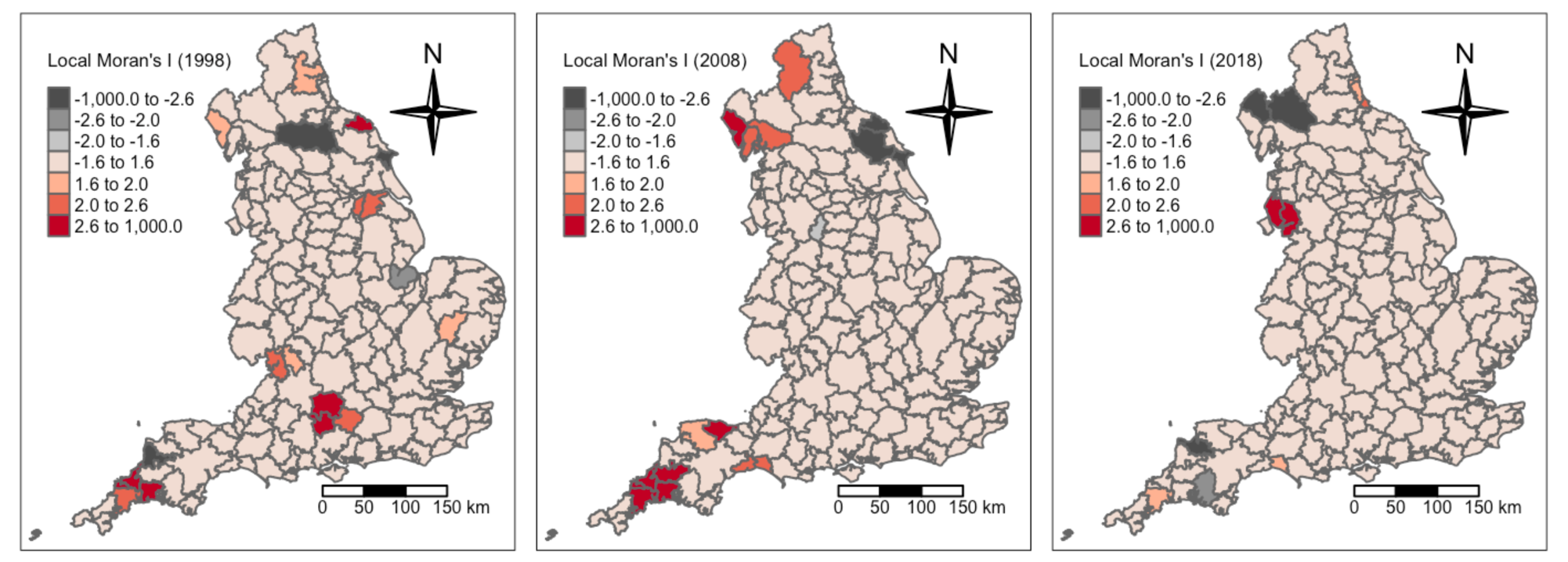
Figure 4.4: Local Moran’s I Spatial Analysis for Entry Rate in England for Three Time Periods
4.3.2 Hot-Spot Analysis of Firms Dynamics
This research identified and mapped local clusters (hot and cold spots) by the level of entry rate for these three period.
On the whole, there is a distinct north-south difference in the distribution of cold and hot spots in the early stage(1998). With the development of England tech clusters, this difference is slowly dissipating and a reversal is formed eventually(Figure 4.5). More specifically, in 1998, there were some hot spots concentrated in the Swindon-Bristol-Reading urban belt in the south-central area and the southwest urban agglomeration of Exeter. Whilst, in the north, there were scattered cold spots represented by the Whitehaven area.
By 2008, most of the hot spots disappeared, and the places that were hot spots gradually became cold spots, such as the southwestern region. In 2018, some hot spots appeared in the northwestern region along with England. The original two hot spots in the southwest have experienced two-time nodes in 2008 and 2018, and they finally turned into cold spot clusters(Figure 4.5).
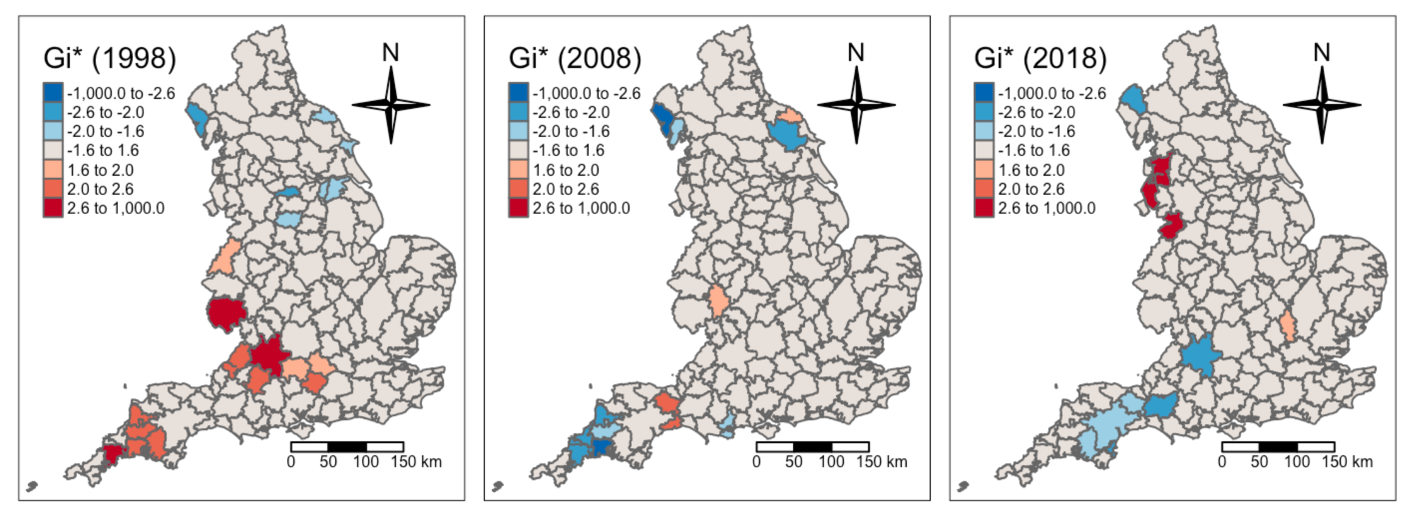
Figure 4.5: Local Gi* Score Statistics for Entry Rate in England for Three Time Periods